DataFrames - Part 1
Figure 1

Figure 2

Figure 3
Figure 4
Figure 5
Figure 6
Figure 7

Figure 8
Figure 9
Figure 10
Figure 11
Figure 12
Figure 13
Data Frames - Part 2
Figure 1
Figure 2
Figure 3
Figure 4
Figure 5
Figure 6
Figure 7
Figure 8
Figure 9
Figure 10
Figure 11
Figure 12
Figure 13
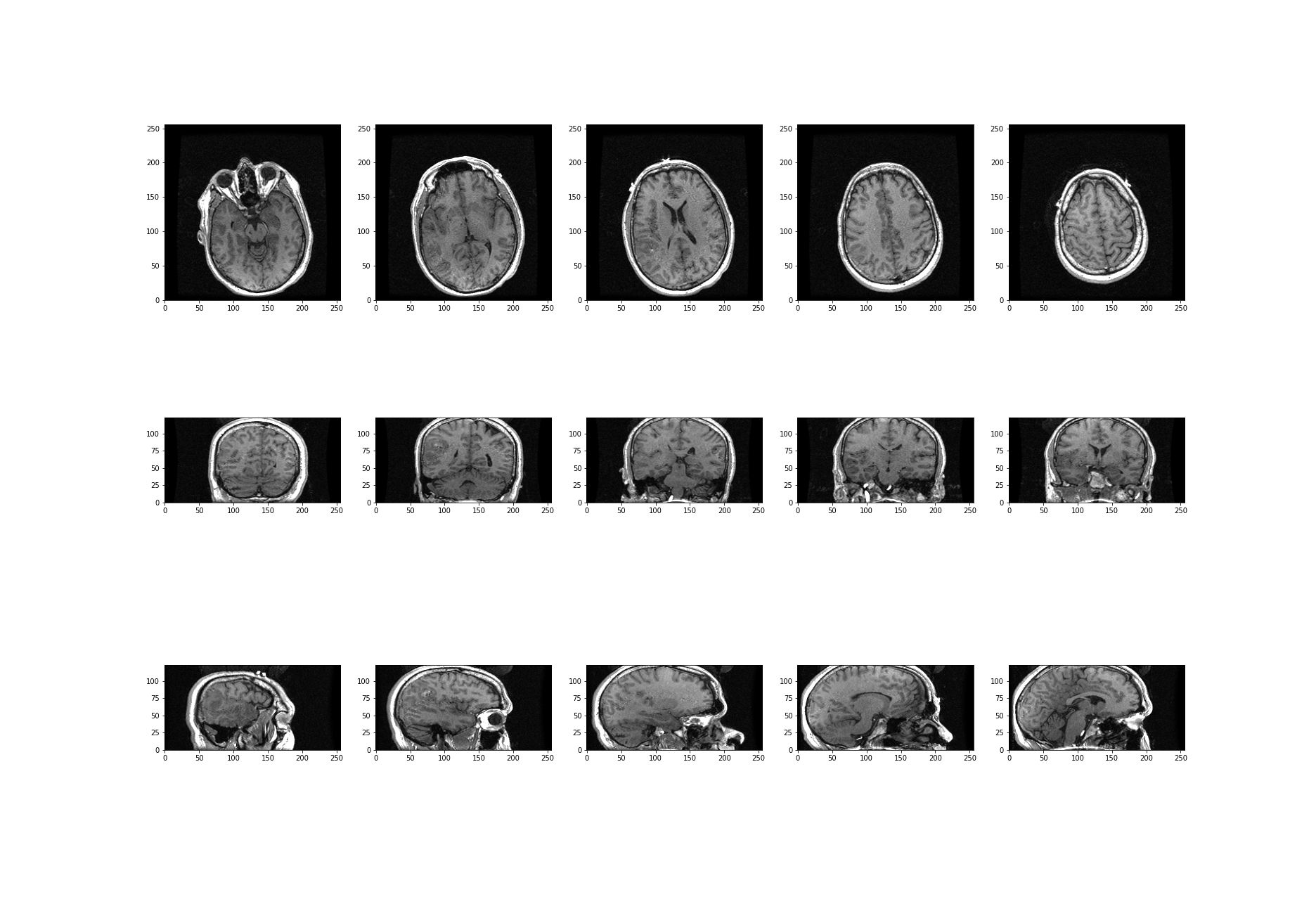
Image Handling
Figure 1
Figure 2
Figure 3
Figure 4
Figure 5
Figure 6
Figure 7
Figure 8
Figure 9
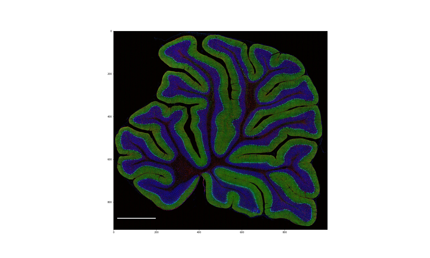
Figure 10
Figure 11
Figure 12

Figure 13
Figure 14
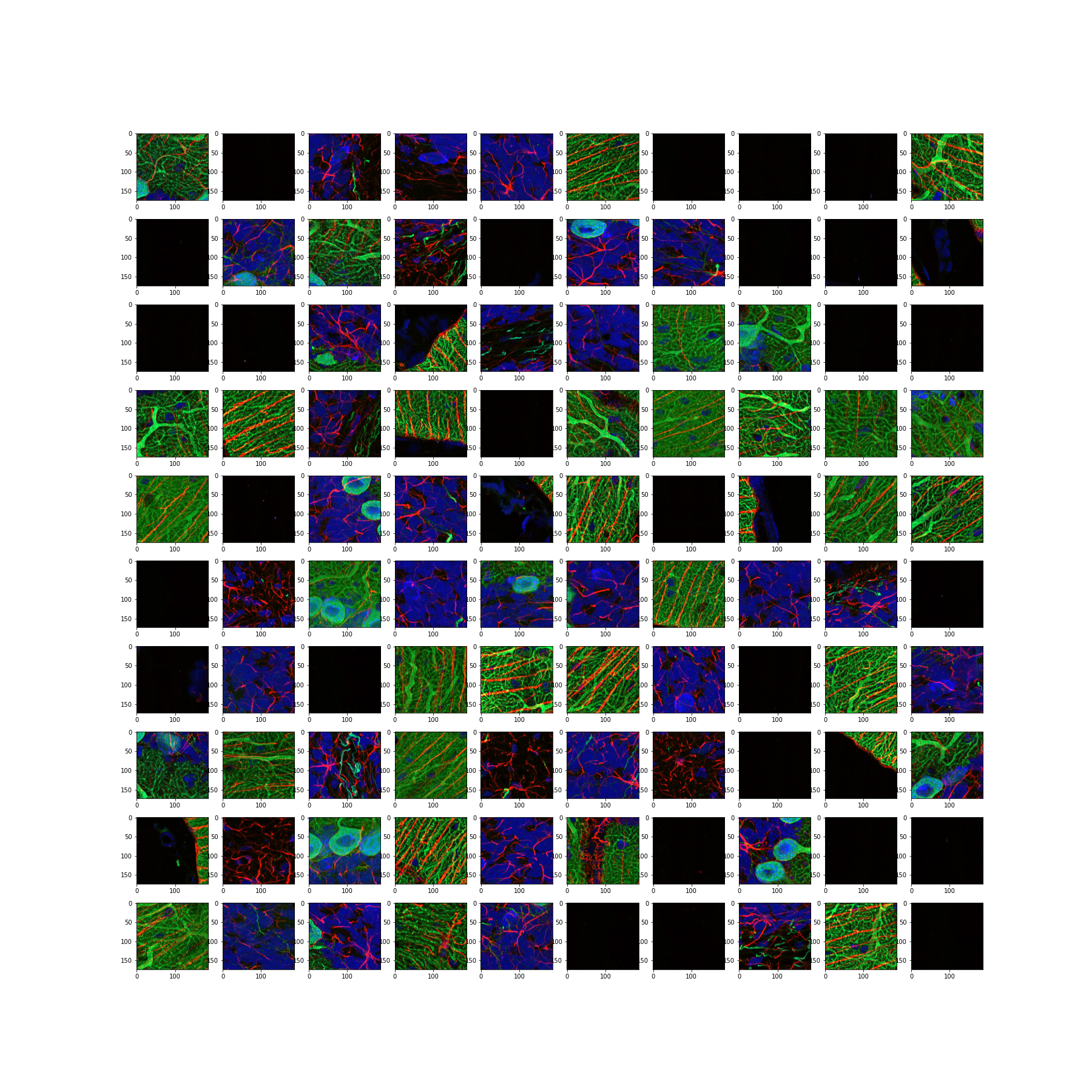
Figure 15
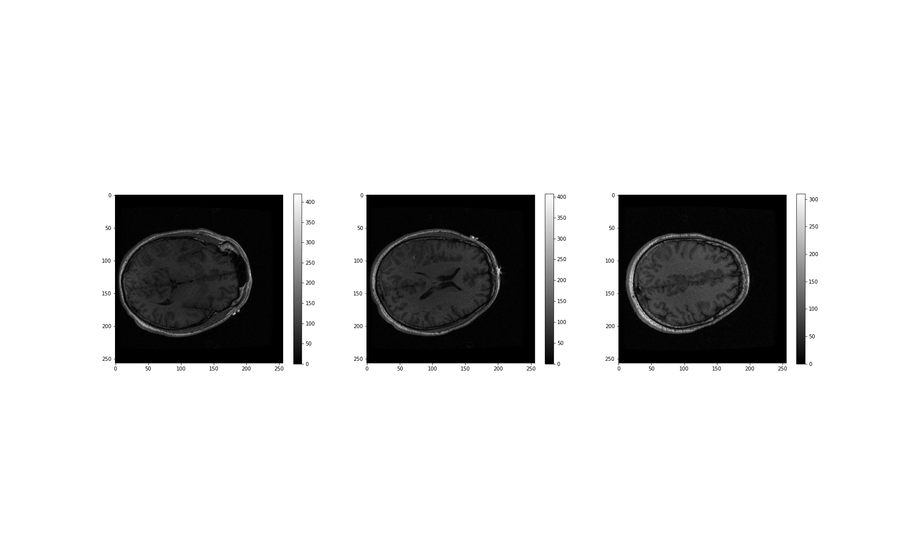
Figure 16
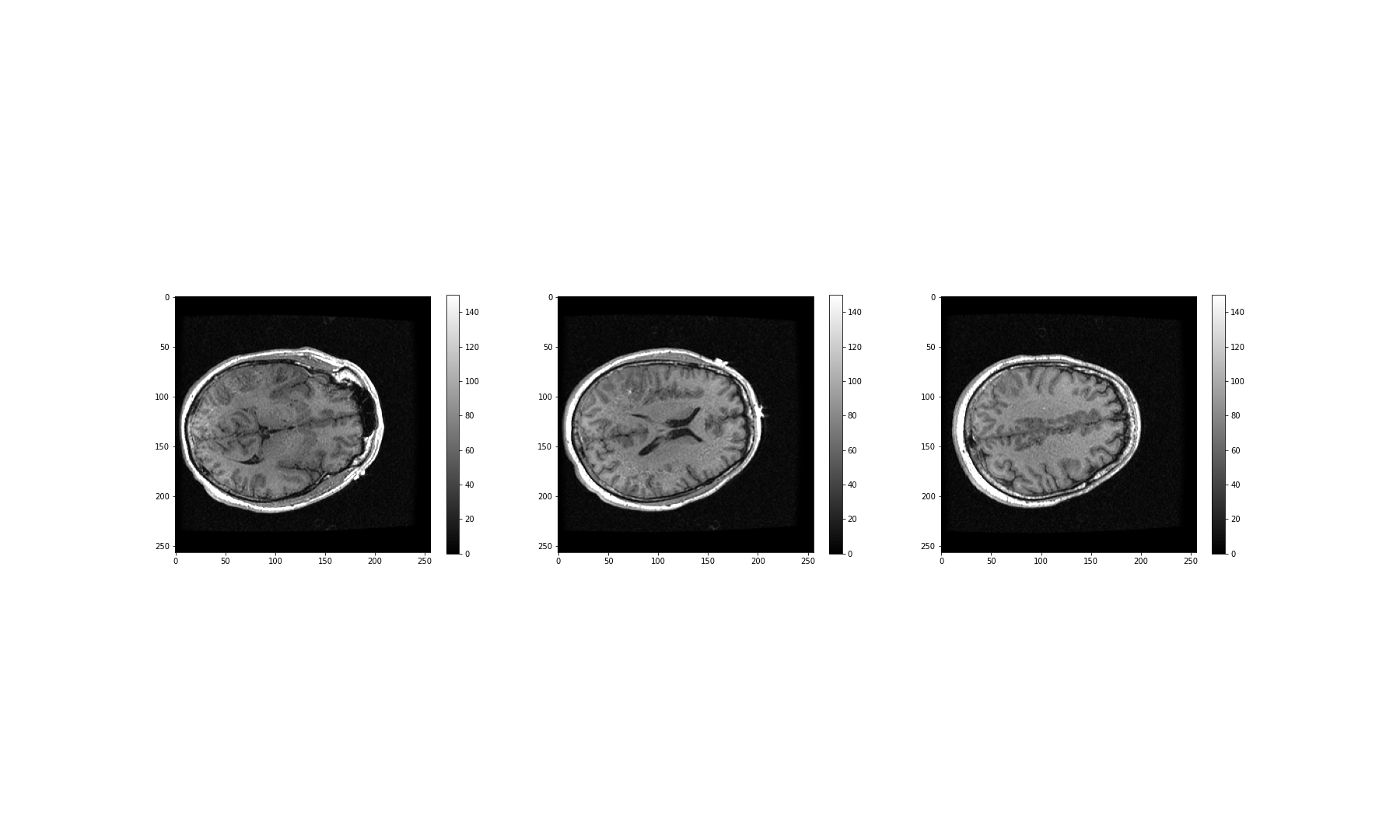
Figure 17
Time Series
Figure 1
Figure 2
Figure 3
Figure 4
Figure 5
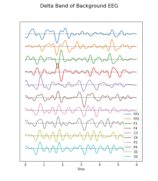
Figure 6

Figure 7
Fourier Transform of EEG data
We import the Fourier Transform function fft from the
library scipy.fftpack where it can be used to transform
all columns at the same time.
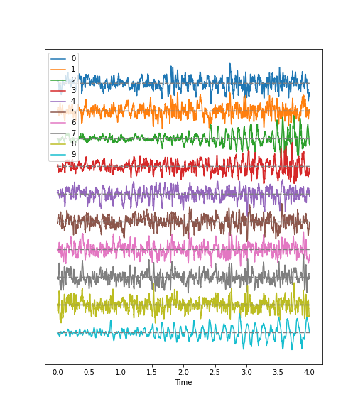
Firstly, we must obtain a Fourier spectrum for every data column. Thus, we need to define how many plots we want to have. If we take only the columns in our data, we should be able to display them all, simultaneously.
Secondly, the Fourier Transform results in twice the number of complex coefficients; it produces both positive and negative frequency components, of which we only need the first (positive) half.
Lastly, the Fourier Transform outputs complex numbers. To display the ‘amplitude’ of each frequency, we take the absolute value of the complex numbers, using the abs() function.
PYTHON
no_win = 2

rows = data_back.shape[0]

freqs = (sr/2)*linspace(0, 1, int(rows/2))

amplitudes_back = (2.0 / rows) * abs(data_back_fft[:rows//2, :2])


fig, axes = subplots(figsize=(6, 5), ncols=1, nrows=no_win, sharex=False)

names = df_back.columns[:2]

for index, ax in enumerate(axes.flat):
    axes[index].plot(freqs, amplitudes_back[:, index])
    axes[index].set_xlim(0, 8)
    axes[index].set(ylabel=f'Amplitude {names[index]}')

axes[index].set(xlabel='Frequency (Hz)');

show()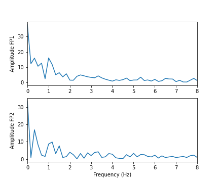
In these two channels, we can clearly see that the main amplitude contributions lie in the low frequencies, below 2 Hz.
Let us compare the corresponding figure for the case of seizure activity:
PYTHON
fig, axes = subplots(figsize=(6, 5), ncols=1, nrows=no_win, sharex=False)

names = df_epil.columns[:2]

amplitudes_epil = (2.0 / rows) * abs(data_epil_fft[:rows//2, :2])

for index, ax in enumerate(axes.flat):
    axes[index].plot(freqs, amplitudes_epil[:, index])
    axes[index].set_xlim(0, 12)
    axes[index].set(ylabel=f'Amplitude {names[index]}')

axes[index].set(xlabel='Frequency (Hz)');

show()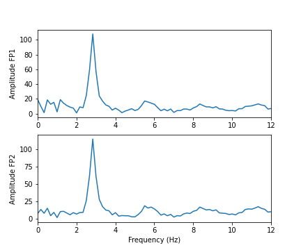
As we can see from the Fourier spectra generated above, the amplitudes are high for low frequencies, and tend to decrease as the frequency increases. Thus, it can sometimes be useful to see the high frequencies enhanced. This can be achieved with a logarithmic plot of the powers.
PYTHON
fig, axes = subplots(figsize=(6, 6), ncols=1, nrows=no_win, sharex=False)

for index, ax in enumerate(axes.flat):

    axes[index].plot(freqs, amplitudes_back[:, index])
    axes[index].set_xlim(0, 30)
    axes[index].set(ylabel=f'Amplitude {names[index]}')
    axes[index].set_yscale('log')

axes[no_win-1].set(xlabel='Frequency (Hz)');
fig.suptitle('Logarithmic Fourier Spectra of Background EEG', fontsize=16);

show()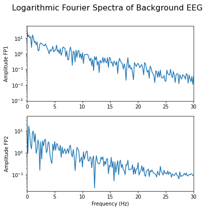
And for the seizure data:
PYTHON
fig, axes = subplots(figsize=(6, 10), ncols=1, nrows=no_win, sharex=False)

for index, ax in enumerate(axes.flat):

    axes[index].plot(freqs, amplitudes_epil[:, index])
    axes[index].set_xlim(0, 30)
    axes[index].set(ylabel=f'Power {names[index]}')
    axes[index].set_yscale('log')

axes[no_win-1].set(xlabel='Frequency (Hz)');
fig.suptitle('Logarithmic Fourier Spectra of Seizure EEG', fontsize=16);

show()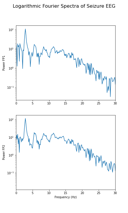
In the spectrum of the absence data, it is now more obvious that there are further maxima at 6, 9, 12 and perhaps 15Hz. These are integer multiples or ‘harmonics’ of the basic frequency at around 3Hz, which we term as the fundamental frequency.
A feature that can be used as a summary statistic, is to caclulate the band power for each channel. Band power is the total power of a signal within a specific frequency range. The band power can be obtained by calculating the sum of all powers within a specified range of frequencies; this range is also referred to as the ‘band’. The band power, thus, is given as a single number.
PYTHON
data_epil_filt = data_filter(data_epil, sr, 4, 12)

data_epil_fft = fft(data_epil_filt, axis=0)

rows = data_epil.shape[0]

freqs = (sr/2)*linspace(0, 1, int(rows/2))

amplitudes_epil = (2.0 / rows) * abs(data_epil_fft[:rows//2, :no_win])

fig, axes = subplots(figsize=(6, 10), ncols=1, nrows=no_win, sharex=False)

for index, ax in enumerate(axes.flat):
    axes[index].plot(freqs, amplitudes_epil[:, index])
    axes[index].set_xlim(0, 12)
    axes[index].set(ylabel=f'Amplitudes {names[index]}')
axes[no_win-1].set(xlabel='Frequency (Hz)');

fig.suptitle('Fourier Spectra of Seizure EEG', fontsize=16);

show()
Figure 8
Figure 9
Figure 10
Figure 11
Figure 12
Figure 13
Figure 14